Drift calculations
Distribution distance functions that yield a single, clear value
Detecting changes in the distribution of a feature, model probability, or any data entity is an important part of the ML process. To track such changes, one could use a long list of statistical parameters such as distribution mean, min value, max value, variance, and more (all available in the product). However, to reduce the noise level and determine whether there was a change, Superwise uses a unique set of distribution distance functions to yield a single, unambiguous value, allowing change to be assessed over time.
Distribution change functions
Distribution change functions quantify the statistical distance (i.e., level of change) between two distributions (or two samples from which the empirical distribution is inferred). Different functions are used for different entity types. The metric scale ranges from 0-100, where 0 indicates identical distribution and 100 indicates orthogonal distribution.
Distribution change for categorical or boolean entities
We use a symmetric chi-square distance function for categorical or boolean data entities.
Definition:

Where P and Q are two distributions or samples of a random variable and P(i) & Q(i) are the probability value in the corresponding sample.
Example:
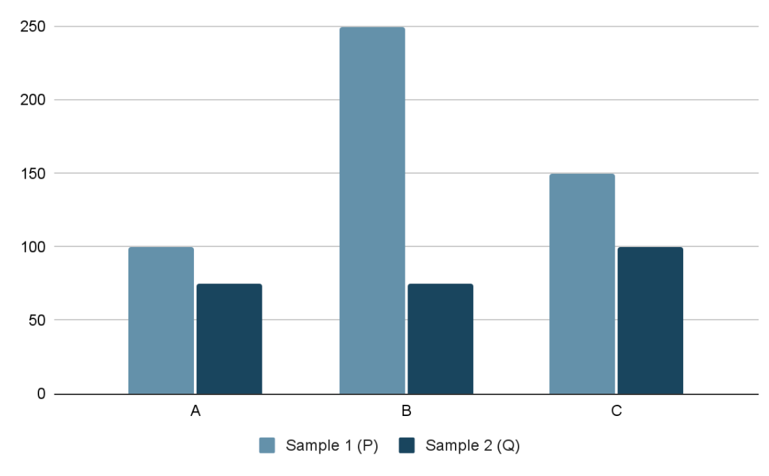
Let's assume we have two samples, P and Q, from some categorical feature with the following distribution:
| Value | Sample 1 (P) | Sample 2 (Q) |
|---|---|---|
| A | 100 (20%) | 75 (30%) |
| B | 250 (50%) | 75 (30%) |
| C | 150 (30%) | 100 (40%) |


Numeric entities:
For numeric data entities, we use a normalized version of the Wasserstein distance function (aka the move earth distance). This distance function quantifies the amount of “work” required to convert distribution P to distribution Q. The Wasserstein distance between the distributions P and Q can be calculated based on their CDFs (cumulative distribution functions):
If U and V are the respective CDFs of P and Q, then

Our calculation is based on scipy implementation with a normalization step to bound the distance to 100. Hence, a distance between two distributions with no overlap will be 100, regardless of the actual distance between the two distributions.
Entity distribution shift
For each entity, we measure the ongoing drift (change level) of the production data from the baseline data. Depending on the configured time-resolution, each time unit is grouped together, and the feature distribution in the time unit is compared with the feature’s distribution in the baseline data.
For example, in daily resolution, the data for each day is grouped, and an empirical distribution is inferred from the data. The distribution is then compared with the feature's distribution in the baseline data, and the drift is measured with the proper drift function (depending on the feature type).
Input drift
Input drift is an aggregate measure of the drifts in all features to a single metric.
Updated over 3 years ago
